Conformal mappings

What is a conformal transformation?

Suppose you wanted to draw a map of the earth on a sheet of paper. Doing so necessarily introduces distortions in distances and shapes. Conformal transformations are mappings that locally preserve angles (and therefore shapes) but not necessarily distances. They are relevant in cartography because they preserve directional information.

In two dimensions, any analytic function of a complex variable (i.e. \(f(z,\bar z)\) such that \(\partial_{\bar z}f=0\)) defines a conformal transformation. The group of conformal transformations in 2d is therefore very large in the sense that it takes an infinite number of parameters to specify one such mapping.

Conformal symmetry in physics

In physics where it’s usually true that the more symmetric a system the simpler its mathematical description, conformal symmetry is very powerful. For example, conformal symmetry allows some 2-dimensional systems to be analytically solved. This is the case of the 2d critical Ising model, which was the topic of my research internship.

Visualizing conformal deformations

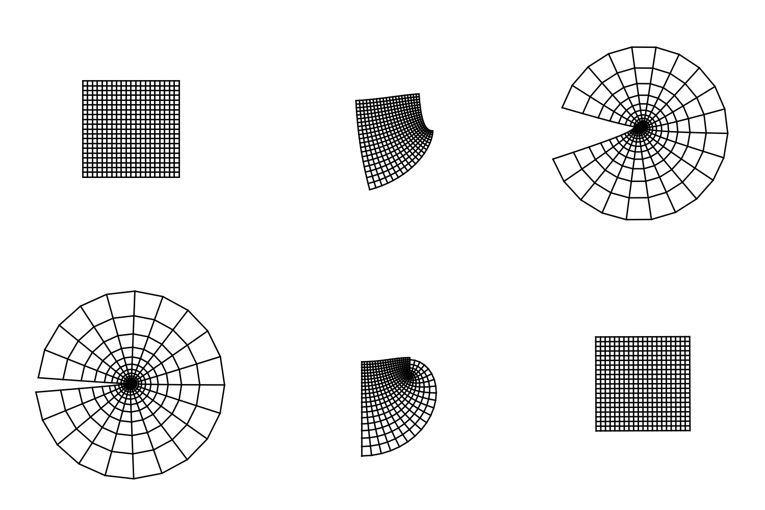
I was curious to visualize conformal deformations of one surface into another. By deformation I mean a continuous set of conformal transformations that takes one surface into another. This can be thought of as a path in the conformal group connecting the identity transformation

to a given conformal transformation, for instance the conformal mapping of the complex plane into an infinite cylinder

One possible path is

This is not the only one but it’s pretty simple and it looks good when animated. You can easily see that \(J(z,\bar z;0) = I(z,\bar z)\) and \(J(z, \bar z; 1) = J(z,\bar z)\). Moreover, for every \(t\in [0,1]\), J is a conformal transformation so this is indeed a path in the conformal group.

The following code creates an animation showing this deformation using the animation library from matplotlib.

import numpy as np
import matplotlib.pyplot as plt
from matplotlib.animation import FuncAnimation

x=np.linspace(-0.5,0.5,21)     #square grid
xx, yy =np.meshgrid(x,x)
Z=xx+1j*yy

## Animation ##

fig = plt.figure()
fig.set_size_inches(5, 5, forward=True)
ax1=plt.axes(aspect="equal")
ax1.set_xlim(-1.02,1.02)
ax1.set_ylim(-1.02,1.02)
ax1.set_xticks([])
ax1.set_yticks([])
ax1.set_axis_off()

lines=[]

for i in range(42):                   #create a line object for each line of the grid
    lobj=ax1.plot([], [], lw=2,c='k',aa=True)[0]
    lines.append(lobj)

def init():
    for line in lines:
        line.set_data([],[])
    return lines

def animate(i):                       #function which evolves the grid of one time step
    a=1.56
    if i <= 20:
        t=np.sin(np.pi*(i/40))**2       #time varies periodically between 0 and 1
    elif i>20 and i <22:                #and stops at t=1 for 1 frame
        t=1
    elif i>= 22:
        t=np.sin(np.pi*((i-2)/40))**2


	#sequence of conformal transformations
    newZ = (1-t)*Z+t*np.exp(2j*t*np.pi*Z)/(np.exp(t*np.pi))  
    
    x = np.concatenate((np.real(newZ),np.transpose(np.real(newZ))), axis=1)
    y = np.concatenate((np.imag(newZ),np.transpose(np.imag(newZ))), axis=1)

    for lnum,line in enumerate(lines):                 #update line by line
        line.set_data(x[:,lnum],y[:,lnum])               
    return lines


anim = FuncAnimation(fig, animate, init_func=init,
                               frames=41, interval=100, blit=True)
anim.save('conformal-deformation.gif', writer='imagemagick')

Output: